Carbon Intensity

import numpy as np
import pandas as pd

import seaborn as sns
import matplotlib.pyplot as plt

Data Preparation

We'll start by loading the dictionary’s attribute data. This data has been automatically extracted from other datasets which have been linked to assets in the dictionary.

attributes_fp = 'https://osuked.github.io/Power-Station-Dictionary/object_attrs/dictionary_attributes.csv'

df_attrs = pd.read_csv(attributes_fp)

df_attrs.head()

attribute	id	value	datapackage	id_type	year	dictionary_id	financial_year
Fuel Type	MARK-1	BIOMASS	https://raw.githubusercontent.com/OSUKED/Dicti...	ngc_bmu_id	nan	10000	nan
Longitude	10000	-3.603516	https://raw.githubusercontent.com/OSUKED/Dicti...	dictionary_id	nan	10000	nan
Latitude	10000	57.480403	https://raw.githubusercontent.com/OSUKED/Dicti...	dictionary_id	nan	10000	nan
Annual Output (MWh)	MARK-1	355704.933	https://raw.githubusercontent.com/OSUKED/Dicti...	ngc_bmu_id	2016	10000	nan
Annual Output (MWh)	MARK-1	387311.364	https://raw.githubusercontent.com/OSUKED/Dicti...	ngc_bmu_id	2017	10000	nan

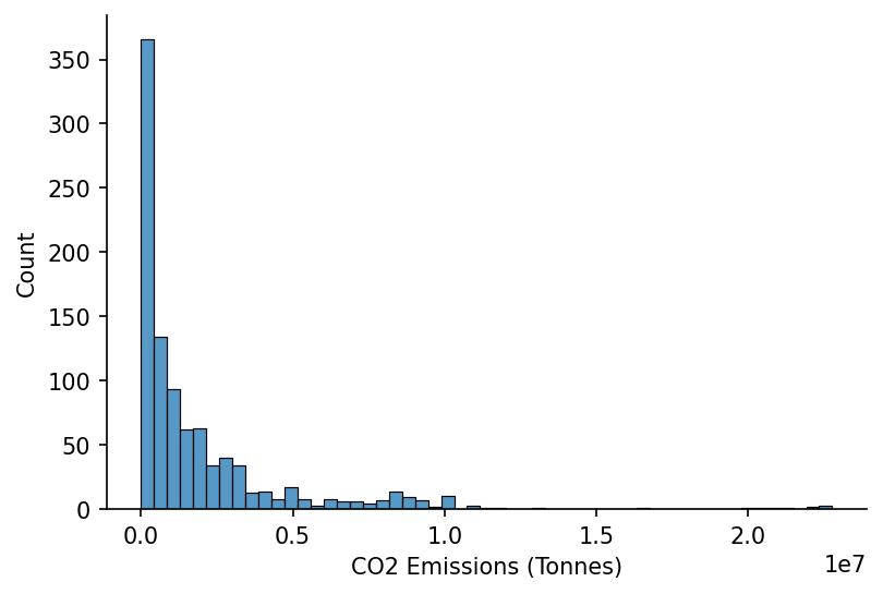
We'll then extract the CO2 emissions data

def hide_spines(ax, positions=["top", "right"]):
    """
    Pass a matplotlib axis and list of positions with spines to be removed

    args:
        ax:          Matplotlib axis object
        positions:   Python list e.g. ['top', 'bottom']
    """
    assert isinstance(positions, list), "Position must be passed as a list "

    for position in positions:
        ax.spines[position].set_visible(False)

co2_attr = 'CO2 Emissions (Tonnes)'

s_site_co2 = (
    df_attrs
    .query('attribute==@co2_attr')
    [['dictionary_id', 'year', 'value']]
    .dropna()
    .astype({'dictionary_id': int, 'year': int, 'value': float})
    .groupby(['dictionary_id', 'year'])
    ['value']
    .sum()
)

# Plotting
fig, ax = plt.subplots(dpi=150)

sns.histplot(s_site_co2, ax=ax)

ax.set_xlabel(co2_attr)
hide_spines(ax)

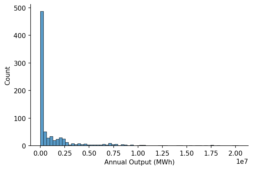
As well as the power output data

output_attr = 'Annual Output (MWh)'

s_site_output = (
    df_attrs
    .query('attribute==@output_attr')
    [['dictionary_id', 'year', 'value']]
    .dropna()
    .astype({'dictionary_id': int, 'year': int, 'value': float})
    .groupby(['dictionary_id', 'year'])
    ['value']
    .sum()
)

# Plotting
fig, ax = plt.subplots(dpi=150)

sns.histplot(s_site_output, ax=ax)

ax.set_xlabel(output_attr)
hide_spines(ax)

And lastly the fuel types of each plant

fuel_attr = 'Fuel Type'

s_site_fuel_type = (
    df_attrs
    .query('attribute==@fuel_attr')
    [['dictionary_id', 'value']]
    .dropna()
    .astype({'dictionary_id': int, 'value': str})
    .groupby('dictionary_id')
    ['value']
    .agg(lambda fuel_types: ', '.join(set(fuel_types)))
)

s_site_fuel_type.value_counts()

WIND                   112
CCGT                    34
NPSHYD                  13
NUCLEAR                  7
OCGT                     4
PS                       4
CCGT, OCGT               3
BIOMASS                  3
COAL, OCGT               1
CCGT, COAL, OCGT         1
Wind                     1
BIOMASS, OCGT, COAL      1
OTHER                    1
Name: value, dtype: int64

Calculating Annual Carbon Intensities

We'll quickly check the data coverage

sites_with_co2_data = s_site_co2.index
sites_with_output_data = s_site_output.index

sites_with_both_datasets = sites_with_co2_data.intersection(sites_with_output_data)

sites_with_co2_data.size, sites_with_output_data.size, sites_with_both_datasets.size

(978, 825, 239)

sites_with_both_datasets.get_level_values(0).unique().size

52

We're now ready to calculate the annual carbon intensities

s_site_carbon_intensity = 1000 * s_site_co2.loc[sites_with_both_datasets]/s_site_output.loc[sites_with_both_datasets]

s_site_carbon_intensity

dictionary_id  year
10002          2016     856.556931
               2017     849.483513
               2018     933.703289
               2019     918.491921
               2020    3368.789243
                          ...     
10104          2016    1104.226297
               2017    1110.856183
               2018    1103.122391
               2019    1125.497186
               2020    1070.007876
Name: value, Length: 239, dtype: float64

We'll identify which sites we also have matched fuel type information for

s_site_fuel_type_mod = s_site_fuel_type.copy()

s_site_fuel_type_mod[s_site_fuel_type.str.contains(', ')] = 'MIXED'
s_site_fuel_type_mod = s_site_fuel_type_mod.replace('Wind', 'WIND')

sites_with_relevant_fuel_types = s_site_fuel_type_mod[s_site_fuel_type_mod.isin(['CCGT', 'OCGT', 'BIOMASS', 'MIXED'])].index

sites_with_relevant_fuel_types.size

47

We'll now filter for only thermal generation

s_site_focus_carbon_intensity = s_site_carbon_intensity.loc[s_site_carbon_intensity.index.get_level_values(0).isin(sites_with_relevant_fuel_types)]
s_site_focus_fuel_types = pd.Series(s_site_focus_carbon_intensity.index.get_level_values(0).map(s_site_fuel_type_mod.to_dict()), index=s_site_focus_carbon_intensity.index)

s_site_focus_carbon_intensity

dictionary_id  year
10004          2016     309.556085
               2017     306.054191
               2018     226.265042
               2019      50.052577
               2020      94.602010
                          ...     
10104          2016    1104.226297
               2017    1110.856183
               2018    1103.122391
               2019    1125.497186
               2020    1070.007876
Name: value, Length: 215, dtype: float64

Finally we're ready to save the dataset

s_site_focus_carbon_intensity.name = 'carbon_intensity_gco2_per_kwh'
s_site_focus_carbon_intensity = s_site_focus_carbon_intensity.replace(np.inf, np.nan).replace(-np.inf, np.nan).dropna()

s_site_focus_carbon_intensity.to_csv('../data/attribute_sources/carbon-intensity/carbon_intensity.csv', float_format='%.2f')

Visualisations

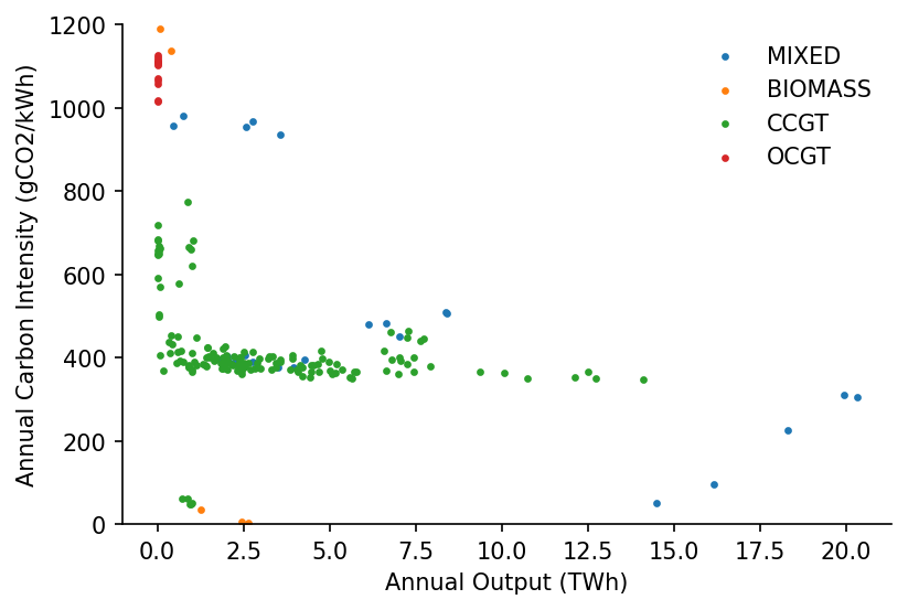
Our first visualisation will be a scatter plot of carbon intensity against annual emissions

fuel_colour_map = {'BIOMASS': 'C1', 'MIXED': 'C0', 'CCGT': 'C2', 'OCGT': 'C3'}

# Plotting
fig, ax = plt.subplots(dpi=150)

for fuel_type in s_site_focus_fuel_types.unique():
    idxs = s_site_focus_fuel_types.index[s_site_focus_fuel_types==fuel_type]
    ax.scatter(s_site_output.loc[idxs].divide(1e6), s_site_focus_carbon_intensity.loc[idxs], c=fuel_colour_map[fuel_type], label=fuel_type, s=5)

hide_spines(ax)
ax.set_ylim(0, 1200)
ax.legend(frameon=False)
ax.set_xlabel('Annual Output (TWh)')
ax.set_ylabel('Annual Carbon Intensity (gCO2/kWh)')

Text(0, 0.5, 'Annual Carbon Intensity (gCO2/kWh)')

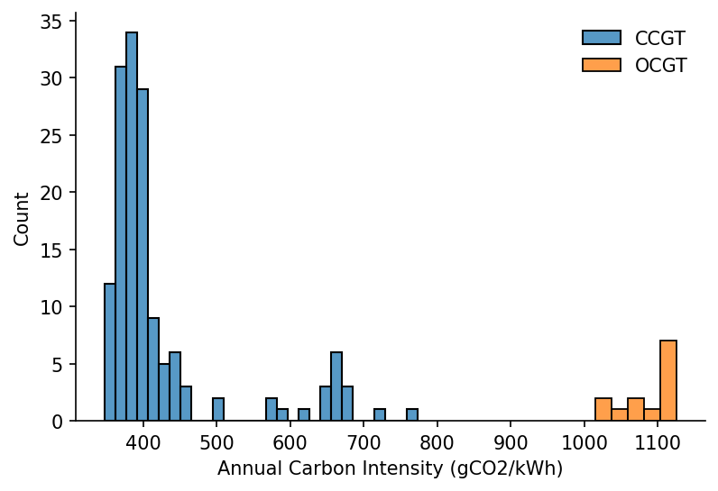
And then create a histogram for only the OCGT and CCGT plants

ccgt_sites = s_site_fuel_type.index[s_site_fuel_type=='CCGT'].intersection(s_site_co2.index.get_level_values(0)).intersection(s_site_output.index.get_level_values(0))
ocgt_sites = s_site_fuel_type.index[s_site_fuel_type=='OCGT'].intersection(s_site_co2.index.get_level_values(0)).intersection(s_site_output.index.get_level_values(0))

s_ccgt_carbon_intensities = 1000*(s_site_co2.loc[ccgt_sites]/s_site_output.loc[ccgt_sites]).dropna()
s_ccgt_carbon_intensities = s_ccgt_carbon_intensities.loc[(s_ccgt_carbon_intensities<1000)&(s_ccgt_carbon_intensities>200)]

s_ocgt_carbon_intensities = 1000*(s_site_co2.loc[ocgt_sites]/s_site_output.loc[ocgt_sites]).dropna()
s_ocgt_carbon_intensities = s_ocgt_carbon_intensities.loc[(s_ocgt_carbon_intensities<1200)&(s_ocgt_carbon_intensities>200)]

# Plotting
fig, ax = plt.subplots(dpi=150)

sns.histplot(s_ccgt_carbon_intensities, ax=ax, label='CCGT')
sns.histplot(s_ocgt_carbon_intensities, ax=ax, color='C1', label='OCGT')

ax.set_xlabel('Annual Carbon Intensity (gCO2/kWh)')
hide_spines(ax)
ax.legend(frameon=False)

<matplotlib.legend.Legend at 0x1e04c6a7b20>